timeseries.tools Blog
Revolutionizing the way businesses analyze time series data.
ArticleSimple moving average (MA) cross-over strategy using the python backtesting libraryIn this post, we will explore a simple moving average (SMA) cross-over strategy for trading financial assets. The strategy is implemented using the backtesting library, which allows us to test our strategy on historical data and evaluate its performance. This is the code. We will go through it step by step. The SMA cross-over strategy is based on the idea that when a short-term SMA crosses above a long-term SMA, it is a signal to buy the asset, and when the short-term SMA crosses below the long-term SMA, it is a signal to sell the asset. This strategy can be implemented in a few lines of code using the backtesting library. First, we import the Backtest and Strategy classes from the backtesting library, as well as the crossover function, which we will use to check for SMA cross-overs: Next, we define a SMA function that calculates the simple moving average of a given series of values. This function takes two arguments: values, which is a list or array of values, and n, which is the number of previous values to take into account when calculating the SMA: Now, we can define our SmaCross strategy class, which subclasses the Strategy class from the backtesting library. The class defines two class variables, n1 and n2, which represent the two moving average lags that are used in the strategy. The init method of the class precomputes the two SMAs using the SMA function, which we defined earlier: The next method of the class is called at each step of the backtesting process and implements the logic of the strategy. If the first SMA crosses above the second SMA, any existing short trades are closed and the asset is bought; if the second SMA crosses above the first SMA, any existing long trades are closed and the asset is sold: Now that we have implemented our SmaCross strategy class, we can use it to test our strategy on some historical data. We will use the Backtest class from the backtesting library to run the backtesting process. First, we need to import the historical data that we will use for the backtesting. In this example, we will use the GOOG data, which is included in the backtesting library and represents the daily closing prices of Google's stock. Next, we create an instance of the Backtest class, passing it the GOOG data, the SmaCross strategy class that we defined earlier, and some additional parameters such as the initial cash balance and the commission rate: Finally, we call the run method on the Backtest instance to run the backtesting process and store the resulting stats in a stats variable: Now that we have run the backtesting process, we can use the stats variable to evaluate the performance of our strategy. The stats variable is a dictionary that contains a variety of metrics and plots that can help us understand how the strategy performed. We can extract the equity curve from it and store it in a equity variable. We can then use the create_tearsheet method of the TimeseriesTools class to create a tearsheet, which is a plot that displays the equity curve and some additional metrics such as the Sharpe ratio and the maximum drawdown. This plot can help us visualize the performance of the strategy and understand how it evolved over time. Our tearsheet will create these graphs! You’ll find the tearsheet here: Also check out some other posts!

Tim David Brachwitz
2022-12-03
6 min read
ArticleCommon pitfalls and challenges in time series analysis and how to avoid them.Time series analysis is a powerful tool for understanding and predicting trends in data that changes over time. However, there are several pitfalls that can lead to inaccurate results and misleading conclusions. In this blog post, we'll discuss some of the most common pitfalls in time series analysis, including non-stationary data, the need for careful data preprocessing, and the use of inappropriate methods or models. We'll also provide tips for avoiding these pitfalls and ensuring the reliability of your time series analysis. By understanding and addressing these challenges, you can improve the accuracy and usefulness of your time series analysis. Those are the top 5 pitfalls:

Parthasarathi Bansal
2022-12-03
6 min read
ArticleThe Variation of a functionIf you want to know the fundamentals of stochastic calculus, you need to know what the variation of a function is. In mathematics, the variation of a function measures how much the output of the function changes as its input changes. This concept is often used in calculus to study the behavior of functions and their derivatives. In simple terms, a function's variation is a measure of how much the output of the function changes as the input changes. For example, if a function always outputs the same value regardless of the input, then we say that the function has zero variation. On the other hand, if the output of a function changes significantly as the input changes, then we say that the function has a high variation. One way to measure the variation of a function is to calculate the average rate of change of the function over a given interval. This is known as the differential of the function, and it measures how much the output of the function changes on average as the input changes. A function with a large average slope has a high variation, while a function with a small average slope has a low variation. Why do we need to know about this? The functions we care about in stochastic analysis (e.g stocks) usually have a really big or infinite variation! This happens when the output of the function changes arbitrarily as the input changes, without any limiting factors. For example, consider the function ⁍ defined over the interval ⁍. This function has a finite range of ⁍, and its derivative ⁍ has a maximum value of ⁍ at ⁍ and a minimum value of ⁍ at ⁍. Therefore, the function ⁍ has a finite variation over the interval ⁍. Now consider the function ⁍. This function also has a finite range of ⁍, but its derivative ⁍ has a maximum value of ⁍ at ⁍ and a minimum value of ⁍ at ⁍. Therefore, the function ⁍ has a higher variation over the interval ⁍ than the function ⁍. However, if we extend the domain of the function ⁍ to include all real numbers, then the derivative ⁍ becomes unbounded. This means that the output of the function ⁍ can change arbitrarily as the input ⁍ changes, without any limiting factors. In this case, we say that the function ⁍ has infinite variation over the interval of all real numbers. In summary, a function can have infinite variation if its derivative is unbounded over the domain of the function. This means that the output of the function can change arbitrarily as the input changes, without any limiting factors. This is the definition of of the total variation for a differentiable function is. This means the Variation of a function is in this case just the arc length of the graph of the function. This is the more general definition: This means we can quantize the domain, sample some random values and add those using Riemann. Calculating the Variation of sin between ⁍ and ⁍: This code generates 1000 random samples of the function f(x) = sin(x) over the interval [0, 2π]. It then plots the samples and the function itself, and computes the total variation of the samples using the formula I provided earlier. Finally, it prints the value of the total variation.
Tim David Brachwitz
2022-12-03
6 min read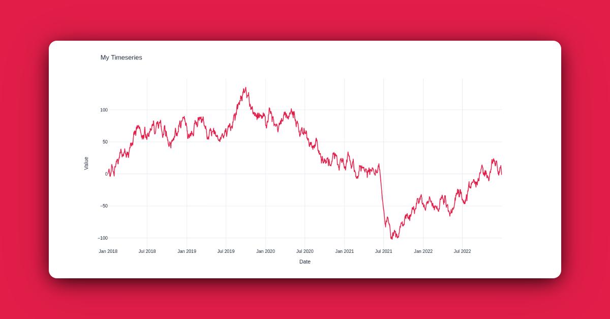
ArticleWhat is a Brownian Bridge?The Brownian bridge is a type of stochastic process that is related to Brownian motion. It is called a "bridge" because it is a stochastic process hat starts at one point, moves randomly according to Brownian motion, and ends at another predefined point. The Brownian bridge is used in many different fields, including finance and engineering, to model the random movement of particles or objects. This is some code that illustrates how it looks like.
Tim David Brachwitz
2022-12-03
6 min read
ArticleGenerate a Brownian Motion in PythonThis code defines two functions, bm_1 and bm_2, which are used to generate and plot Brownian motion samples. The generate_brownian_motion function is a helper function that generates a single Brownian motion sample. It takes two arguments, simulation_time and num_timesteps, which represent the total time of the simulation and the number of timesteps to split the simulation time into, respectively. First, the function calculates the variance of the noise at each timestep by dividing the simulation_time by the num_timesteps. It then generates num_timesteps random normal samples with the calculated variance. Next, it sets the first element of the noise array to 0 and calculates the Brownian motion by summing the noise cumulatively. Finally, it returns the calculated Brownian motion. The bm_2 function generates and plots multiple Brownian motion samples. It takes three arguments: num_samples (the number of Brownian motion samples to generate), simulation_time (the total time of the simulation), and num_timesteps (the number of timesteps to split the simulation time into). First, the function initializes the minimum and maximum values of the Brownian motion to very large/small values. It then generates num_samples Brownian motion samples using the generate_brownian_motion function. For each sample, it generates an array of equally spaced values from 0 to simulation_time. It then plots the Brownian motion and updates the minimum and maximum values if necessary. After generating and plotting all of the samples, the function generates a caption for the plot with the minimum and maximum values of the Brownian motion and sets the title and labels for the plot. Finally, it saves the plot to a file and displays it on the screen. The bm_1 function is similar to bm_2, but it generates and plots only a single Brownian motion sample. It takes no arguments and sets the simulation time and number of timesteps to default values. It then generates a Brownian motion sample using the generate_brownian_motion function, generates an array of equally spaced values from 0 to the simulation time, calculates the minimum and maximum values of the Brownian motion, plots the Brownian motion, generates a caption for the plot with the minimum and maximum values of the Brownian motion, sets the title and labels for the plot, saves the plot to a file, and displays it on the screen. At the end of the code calls the bm_1 and bm_2 functions to generate and plot the Brownian motion samples.
Tim David Brachwitz
2022-12-04
6 min read
Articletimeseries.tools - pyfolio alternativeAre you looking for an alternative to pyfolio? Pyfolio is a popular open-source library for performance and risk analysis of financial portfolios, but it got discontinued. In fact, using a SaaS (Software as a Service) solution can offer several benefits compared to pyfolio, including enhanced features, a user-friendly interface, and ongoing support. One SaaS that offers a compelling alternative to pyfolio is timeseries.tools. timeseries.tools is a powerful tool that helps financial analysts and investors analyze and manage their portfolios. It offers a variety of features, including portfolio and backtest analysis, tear sheets, and risk profiling. But don't just take our word for it – timeseries.tools has helped many financial analysts and investors improve their portfolio analysis and management. If you're looking for an alternative to pyfolio, give timeseries.tools a try. It's easy to use and offers a wealth of features to help you analyze and manage your financial portfolios. Try it out today and see the difference it can make for your portfolio analysis and management. These are the some of the plots that are supported by timeseries.tools.
Parthasarathi Bansal
2022-12-04
6 min read
ArticleExploring three Common Trading Strategies for Algorithmic TradingAlgorithmic trading has become increasingly prevalent in the financial world, with estimates suggesting that between 70-80% of trading volume in the US is generated through algorithms. If you're interested in entering the world of automated trading, it's important to familiarize yourself with some common trading strategies. One way to classify trading strategies is based on whether they are momentum-based or mean-reversion based. Momentum-based strategies are based on the idea that an asset's momentum, if it is going up, will continue to do so. This means that if the momentum slows down, it may be time to exit your position. Mean-reversion, on the other hand, refers to the theory that prices will eventually return to an average if they deviate from it. One popular trading strategy is signal detection, which involves looking for pre-determined criteria to indicate whether a security should be bought or sold. This can be based on technical indicators such as the RSI, MA, MACD, and OBV. Another strategy is pairs trading, which involves trading two stocks in the same sector in the hopes of profiting from their price movements. Another strategy is arbitrage, which involves buying and selling the same asset in different markets in order to profit from price differences. This can be a complex and risky strategy, so it's important to thoroughly research and understand the markets before attempting it. Pairs trading: This involves trading two stocks in the same sector in the hopes of profiting from their price movements. For example, if one stock in the sector is underperforming, a pairs trader might short it and go long on the stock that is outperforming. Ultimately, the strategy you choose will depend on your trading goals and horizon. Momentum-based strategies tend to perform better in the long run, while mean-reversion is more successful in the short run. It's important to conduct your own research and carefully consider which strategy is best suited to your needs.
Parthasarathi Bansal
2022-12-04
6 min read
ArticleVisualizing the Reflection Principle for the Brownian MotionThe reflection principle is a property of Wiener processes, also known as Brownian motion. It states that, if a Wiener process hits a certain point, then the process starting at that point and moving in the opposite direction is a Wiener process with the same distribution as the original process. In other words, if a Wiener process starting at time 0 hits a point at time t, then the process reflected across that point at time t has the same distribution as the original process. This property is called the reflection principle because it is similar to the reflection of a light ray across a mirror.
Tim David Brachwitz
2022-12-04
6 min read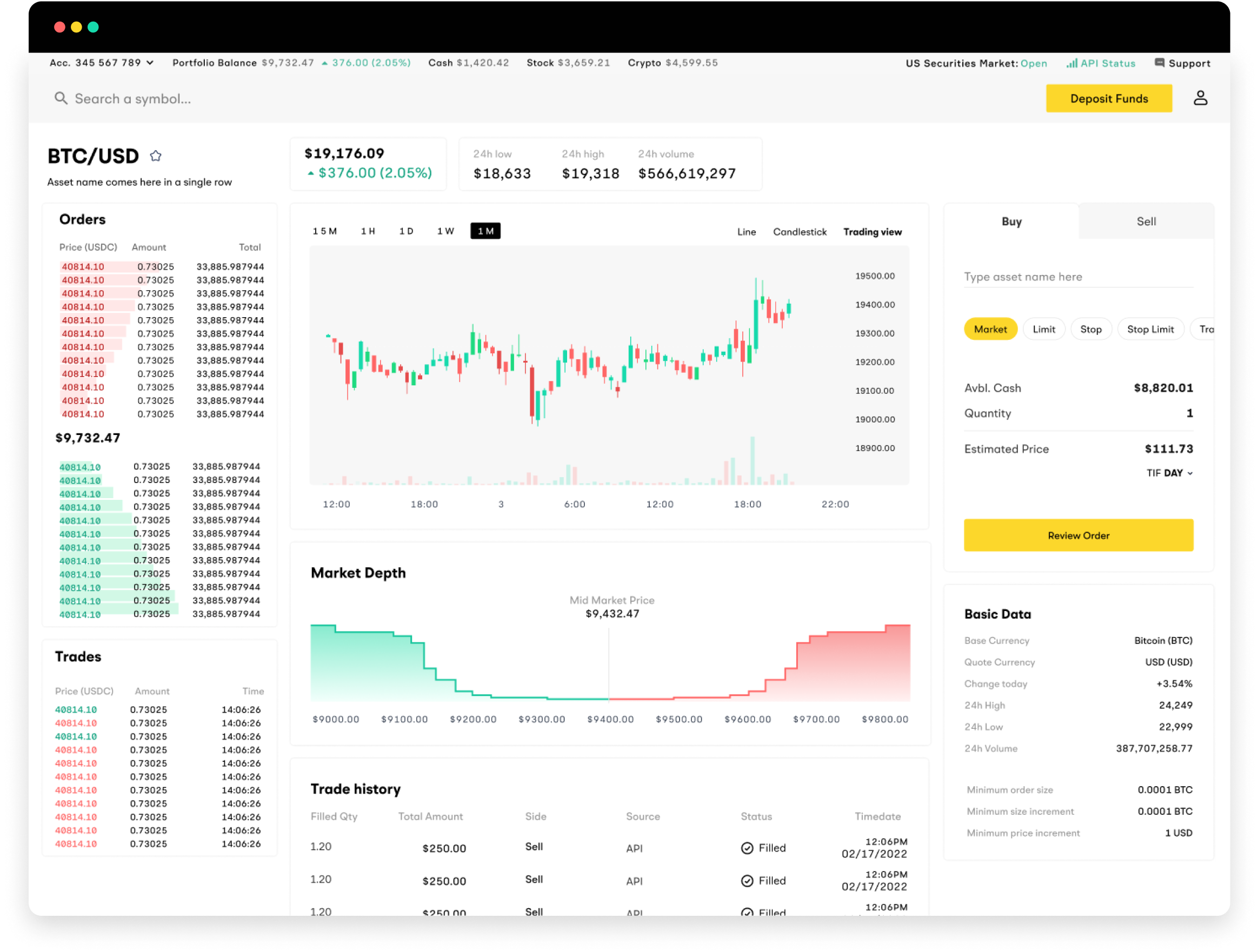
ArticleHow to use alpaca.markets with timeseries.toolsTo use alpaca.markets with timeseries.tools, you can follow these steps: With these simple steps, you can easily use alpaca.markets and timeseries.tools to analyze and track the performance of your chosen stock.
Parthasarathi Bansal
2022-12-04
6 min read